Bracketing is a general technique of taking several shots of the same subject using different camera settings like exposure, sensitivity, white balance, focus or depth of field. This technique is used to accomplish one of the following objectives:

1. When it is difficult to obtain a good image with a single shot (even the most sophisticated automated cameras may fail to get it right in some situations); you will decide in the end which one is the best.
2. When you can combine multiple images into another one with improved qualities that a camera cannot produce directly; the procedure is usually done in post processing using a computer and special software dedicated to this task.

Bracketing cannot be applied for every type of photography, especially in the second case. The time required to take multiple shots makes it almost impossible to use bracketing for anything else other than static scenes. As consequence, wherever there is motion you have only one shot to get it right.

Probably the most common type of bracketing is exposure bracketing. The idea is simple: the camera will determine the normal exposure used as reference and you take at least 3 shots – one normal, one slightly underexposed and one slightly overexposed. You can do it manually or you can use the camera auto-exposure bracketing (AEB) mode (if available) to do it automatically. In either case, the best results are obtained with a camera mounted on a tripod and taking the shots as quickly as possible (the faster the better) to prevent motion blur later in post processing.

The most practical range for exposure bracketing is probably ±2 EV but some cameras may provide either an extended range (e.g. ±3 EV) or a narrower range (e.g. ±1 EV). The number of shots taken is probably 3 is most cases but some cameras (especially the professional ones) will allow bursts of 5 or 7 shots in AEB mode.

Here is a typical screen of a compact camera allowing 3 shots AEB in ±1 EV range:

With this camera you have the following options: ±1/3 EV, ±2/3 EV and ±1 EV. For example, selecting ±2/3 EV (see below)

will produce a set of three images like in the following example:

Panasonic Lumix TZ5, ISO 100, F4.7, 1/100 s: EVa = 11.1, EVr = 0, EVc = 0

Panasonic Lumix TZ5, ISO 100, F4.7, 1/160 s: EVa = 11.78, EVr =2/3, EVc = –2/3

Panasonic Lumix TZ5, ISO 100, F4.7, 1/160 s: EVa = 10.37, EVr = –2/3, EVc = 2/3

In the image captions I used the following notation:

• EV_a is the absolute exposure value corresponding to the current combination of aperture and shutter speed;
• EV_r is the relative variation from the normal (reference) exposure – always 0 for the first image in the AEB set (“the reference image”);
• EV_c is the exposure compensation (or bias) applied to the reference before taking the photo – always 0 for the first image in the AEB set (“the reference image”).

The EV_a value can be calculated from the aperture number and the exposure time (see the “Exposure value” article in Wikipedia). As we mentioned before, this number is less important to be known; in practice, we need to remember the EV_c value (compensation or bias) that indicates if the image will be deliberately underexposed (EV_c is negative) or overexposed (EV_c is positive). Remember: it is our decision to change the default exposure of the camera for two of the images in the AEB set.

The same example shows the most common usage of AEB: taking shots for selecting later which one is better. The decision may be a bit difficult in this case because the first image seems to be the best one anyway. “Why would we need AEB after all?” you may ask.

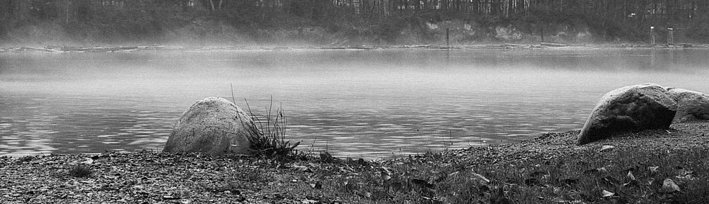
Well, take a look at the water in all three situations. In the reference image the texture of the water is barely visible, in the underexposed one the water is realistic (you can easily see the ripples created by wind) and in the overexposed image the water is completely washed out. If the final result should represent the water realistically, we will need to select the “underexposed” image and work in post processing later (using a computer) to correct the exposure only for the foliage of the tree while keeping the water details intact. The final result may look like in the following image:

Post processed image obtained from the underexposed one in the AEB set

While not perfect, this photo is probably better than any individual one we have in the set. When it comes to post processing, there are a lot of tools that can produce even better results.

One more note: the three image AEB set we’ve got cannot be used to accomplish the second goal – the image combination. Some may say that you can take whatever is good in each image to compose a better image and this is true but not in this example. The image set was taken with a handheld camera (i.e. no tripod) in a relatively windy day (the leaves were moving – i.e. not a static image).

The AEB images produced from static scenes are the main ingredient in obtaining HDR (High Dynamic Range) photos. We will examine HDR separately later in a set of future posts dedicated to this subject.

The next post will be dedicated to histograms. Why is this subject important? The histogram, if properly understood, can be a very useful tool in analyzing the exposure of the image and assisting the photographer to take the right decision even in situations where the automated algorithms in the camera fail.